
A tile’s strength is a numerical representation of how much weight the tile can support before breaking. The results are expressed in N and they may be converted into kg/cm2 using the dimensions of each tile. We are going to go over some methods that can be used to determine a tile’s strength.
To determine the flexural strength of a tile composition in a lab, it is necessary to break a number of tiles of the same composition to calculate an average value or the mean. The higher the number of replicates, the higher the accuracy of the average value obtained. However, measuring a high number of replicates per composition requires investing more time and a higher amount of raw materials. Therefore, in the end the number of replicates per composition shall be a compromise between accuracy and the availability of time & raw materials.
But how to find that optimum compromise value? Statistical tools like the estimation of the confidence limits for the mean (Snedecor and Cochran, 1989) may help us finding the optimum number of replicates per composition. The width of the interval gives us an idea about the uncertainty associated to the mean calculation. It is necessary to consider a determined probability, commonly 95%, to estimate the confidence limits.
The confidence limits for the mean can be calculated following a standard UNE 66040, equivalent with International Standard ISO 2602:1980. To determine them, taking a confidence level of 1-α, the following equation is used:
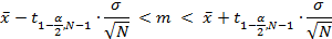
Where  is the t of students, α is the confidence level, ϭ is the standard deviation, N is the number of tiles broken and
 ![]() is the average value.
is the average value.
For a typical flexural strength of 30 kg/cm2, the following figure shows how confidence limits for the mean change with the number of replicates per composition. Different values of the standard deviation were considered in the calculation.
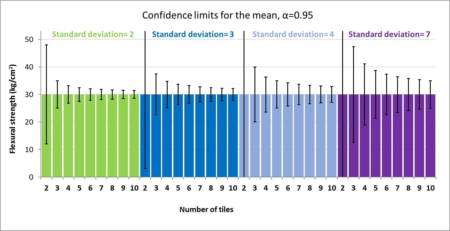
As can be seen in the graph above, the confidence limits calculated are really wide in case of breaking a low number of tiles, i.e. 2, and they become more narrow with the increasing number of replicates. On the other side, the higher the standard deviation, the wider the confidence limits.
Based on laboratory experience, the typical standard deviation is around 4, and the number of replicates is around 6 or 7 to gain a suitable accuracy of the strength values. A higher number of replicates would not be worthwhile because it would not provide significant reduction of confidence limits, and it would require investing more time and necessitate a higher amount of raw materials.
Many statistical techniques are sensitive to the presence of outliers. The mean calculations or the standard deviation may be affected by data too high or too low resulting from experimental error. To avoid these extreme variations that can distort the average, the outliers of each composition have to be detected and removed, and the statistical confidence limits recalculated. Checking for outliers should be a routine part of any statistical analysis. There are some methods to detect outliers:
- Grubbs test
- Tietjen-Moore test
- Generalized extreme derivate test
Grubbs’ test is used to detect a single outlier in a univariate data set that follows an approximately normal distribution (Grubbs, 1969 and Stefansky, 1972). If Gi > Glimit, this datum is considered an outlier and it would be removed and the statistical confidence limits would be recalculated.
Test Statistic: The Grubbs’ test statistic is defined as:
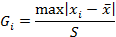
Where ![]() is the average value and S is the standard deviation.
is the average value and S is the standard deviation.
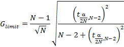
Where N is the number of tiles broken, ![]() is the t of students and α is the confidence level, usually 0.05.
is the t of students and α is the confidence level, usually 0.05.
The Tietjen-Moore test is used to detect multiple outliers in a normal distribution (Tietjen and Moore, 1972). It is important to note that this test requires that the suspected number of outliers be specified exactly. The numbers have to be classified from smaller to the largest and the outliers will be identified in the extreme data, the lowest or/and the highest. If this is not known, it is recommended to use the generalized extreme derivate test instead.
The generalized extreme derivative test (Rosner, 1983) is used to detect one or more outliers in a univariate data set that follows an approximate normal distribution. This method is basically the Grubbs test applied sequentially to detect more than one outlier after deleting the first one. The difference between them is that this new method considers the possibility to have more than one outlier at the beginning and it makes some adjustments for the critical values. It is possible that Grubbs test only detects one outlier while the generalized extreme derivate tests find more.